Urban planner Jarrett Walker emphasizes the importance of transit frequency:

Transit frequency is the elapsed time between consecutive buses (or trains, or ferries) on a line, which determines the maximum waiting time. People who are used to getting around by a private vehicle (car or bike) often underestimate the importance of frequency, because there isn’t an equivalent to it in their experience. A private vehicle is ready to go when you are, but transit is not going until it comes. High frequency means transit is coming soon, which means that it approximates the feeling of liberty you have with your private vehicle – that you can go anytime. Frequency is freedom!

This makes intuitive sense. Transit networks with higher frequency and shorter waiting times will yield a more reliable and empowering experience for passengers than those with lower frequency and longer waiting times.

Analyzing transit frequency in an intuitive way, however, can be difficult. Static transit maps provide geographic context but do not give any information about frequency. Timetables provide information about frequency but can be overwhelming, unintuitive and lacking geographic context. Perhaps we can use spatial-temporal visualization to combine the spatial information of a static transit map with the temporal information of a timetable, and make it easer to think and talk about transit frequency!

This is the motivation behind TransitFlow, an experimental set of tools to generate spatial-temporal transit frequency datasets and visualizations from the command line.

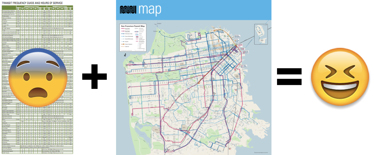
Mmmm… timetables. Provided by the San Francisco Municipal Transportation Agency.

TransitFlow consists of two parts:

1. A few python scripts to retrieve and wrangle transit schedule data from Transitland, an open-source data service sponsored by Mapzen that aggregates transit network data from around the world. Transitland enables us to merge transit schedules from different operators without having to worry about the granular details of each operator’s GTFS data.

2. A template to generate a Processing sketch to animate that data.

Let’s look at a few examples of what you can do with TransitFlow.

Bay Area

• python transitflow.py --name=bay_area --bbox=-123.280334,37.011326,-120.607910,38.955137 --clip_to_bbox

San Francisco

• python transitflow.py --name=san_francisco --bbox=-122.515411,37.710714,-122.349243,37.853983 --clip_to_bbox

Chicago

• python transitflow.py --name=chicago --bbox=-87.992249,41.605175,-87.302856,42.126747 --clip_to_bbox

Mexico City

• python transitflow.py --name=mexico_city --bbox=-100.041504,18.453557,-97.701416,20.040450 --clip_to_bbox --date=2016-06-01

Many more examples available here.

How it works

Getting the data

TransitFlow makes use of three Transitland API endpoints to get the data:

1. Stops to get transit stop locations
2. Routes to get operator vehicle types
3. ScheduleStopPairs to get origin -> destination schedule stop pairs

The ScheduleStopPairs endpoint does the bulk of the work. Each ScheduleStopPair is an edge between an origin stop and a destination stop. Each ScheduleStopPair includes origin departure time and location, destination arrival time and location, and a service calendar which tells you which days a trip is possible. TransitFlow searches for all ScheduleStopPairs for a specified operator or for many operators within a specified bounding box. It then parses the data, calculates trip durations and bearings, and concatenates everything into a tidy, tabular dataset. It then outputs this dataset to single CSV file, which will drive the animation.

Visualizing the data

TransitFlow generates a Processing sketch file based on your command line arguments. The Processing sketch reads in the CSV file from the previous step, uses the Unfolding Maps library to load map tiles and convert geolocations into screen positions, and animates vehicle movements from origin stop to destination stop using linear interpolation. (Note that we are animating between stops and not yet following the exact route line.)

How to use it

First, navigate to the github repository and follow the relatively painless set-up instructions.

You can visualize a single transit operator by passing in the operator’s Onestop ID as a command line argument. What’s a Onestop ID, you ask? As part of Transitland’s Onestop ID Scheme, every transit operator, route, feed and stop are assigned a unique identifier called a Onestop ID. You may look up an operator’s Onestop ID using the Transitland Feed Registry.

For example, the onestop ID for San Francisco BART is o-9q9-bart. To visualize BART’s schedule on today’s date: python transitflow.py --name=bart --operator=o-9q9-bart

You can also visualize many operators within a region by passing in your bounding box of interest as a command line argument. I like using bboxfinder to draw a bounding box. The bounding box must be in the format: West, South, East, North. For example, to visualize Portland transit flows on today’s date: python transitflow.py --name=portland --bbox=-123.035889,45.257489,-122.250366,45.798170 --clip_to_bbox

To view your transit visualization, navigate to sketches\{name}\{date}\sketch and open the sketch.pde file. This should open the Processing application. Simply click the play button or command + r to run the animation.

Command line arguments

Key	Status	Description	Example
--name	required	The name of your project	--name=boston
--date	optional	Defaults to today’s date	--date=2017-08-25
--operator	optional	Operator onestop_id	--operator=o-drt-mbta
--bbox	optional	West, South, East, North	--bbox=-71.4811,42.1135,-70.6709,42.6157
--clip_to_bbox	optional	Clip results to bounding box	--clip_to_bbox
--exclude	optional	Operators to be excluded	--exclude=o-9-amtrak
--apikey	optional	Mapzen API key	--apikey=mapzen-abc1234

Map with us

If you use this tool, we’d love you hear from you! Share your visualizations by tagging @transitland on Twitter or reaching out to us at hello@mapzen.com.

We’re thinking about ways to make this better!

• We would like to add points between stops to make routes with curves and sharp turns smoother at high zooms.
• The animation does not take into account train length or passenger load – if you know of open data sources with this information, let us know!
• We are investigating the best ways to introduce time controls for different start and stop times.
• Real-time data is a longer-term goal for Transitland.

If you have any other suggestions for features, please file an issue in the Github repo.

And as a reward for those of you who read all the way to the bottom of this post, here’s Bay Area transit set to Claude Debussy’s Clair de Lune:

Bay de Lune from Mapzen on Vimeo, Clair de Lune by Claude Debussy, via Dreamnote Music