Welcome back! This is our third installment of a new series that we are calling Make Your Own. If you’ve missed the last two, I recommended giving those a read, as they lay the groundwork for getting started with mapzen.js and the Tangram scene file:
Last time, I showed you how to make a map sandwich by inserting your data layer in between the other map layers displayed on the map. This resulted in labels on top (and, if you are anything like me, a whole lot of celebratory dancing 💃).
This week, we’ll push our map sandwich even further by setting up filters and using JavaScript to create a custom style for our data.
Let’s jump right in, shall we?
Note: The following instructions assume you have a text editor and access to a web server. If you need either, read our documentation on setting up a bare bones development environment or use the gist → bl.ocks workflow described in One Minute Map.
We’ll start with the same two files we created last time, with some minor changes to our national park polygons.
index.html:
<!DOCTYPE html>
<html lang="en">
  <head>
    <title>San Juan Island Geology</title>
    <meta charset="utf-8">
    <link rel="stylesheet" href="https://www.nextzen.org/js/nextzen.css">
    <script src="https://www.nextzen.org/js/nextzen.min.js"></script>
    <style>
      #map {
        height: 100%;
        width: 100%;
        position: absolute;
      }
    html,body{margin: 0; padding: 0}
  </style>
  </head>
  <body>
    <div id="map"></div>
    <script>
      // Mapzen API key (replace key with your own)
      // To generate your own key, go to https://mapzen.com/developers/
      L.Mapzen.apiKey = 'mapzen-JA21Wes';

      var san_juan_island = [48.5326, -123.0879];

      var map = L.Mapzen.map('map', {
        center: san_juan_island,
        zoom: 12,
        scene: 'scene.yaml',
      });

      // Move zoom control to the top right corner of the map
      map.zoomControl.setPosition('topright');

      // Mapzen Search box (replace key with your own)
      // To generate your own key, go to https://mapzen.com/developers/
      var geocoder = L.Mapzen.geocoder('mapzen-JA21Wes');
      geocoder.addTo(map);

    </script>
  </body>
</html>
UPDATE March 1, 2017: A Mapzen developer API key is now required for mapzen.js. We’ve updated the Make Your Own series to include a demo key. Generate your own free API key at https://mapzen.com/developers/.
scene.yaml:
import: https://mapzen.com/carto/refill-style/6/refill-style.zip

sources:
    _nps_boundary:
        type: GeoJSON
        url: https://gist.githubusercontent.com/rfriberg/684645c22f495b4a46f29fb312b6d268/raw/843ed38a3920ed199082636fe198ba995f5cfc04/san_juan_nhp.geojson

layers:
    _national_park:
        data: { source: _nps_boundary }
        draw:
            lines:
                visible: false
                width: [[8, 0.5px], [18, 5px]]
                color: '#518946'
                order: global.sdk_order_under_roads_1
Notice that we removed the polygons, but kept the boundary lines. Though, if you view the map now, the lines won’t display because we set visible: false. We’ll come back to those later.
As before, we are going to focus on San Juan Island in Washington. While San Juan is best known for that time when the U.S. and Great Britain nearly went to war over the death of a pig, we’re going to take a look at the island’s geology. (I’ll try to keep the rock puns to a minimum.)
The geology dataset we will be using began its journey as a shapefile of polygons representing geologic units for San Juan Island, downloaded from Data.gov. Currently, Tangram supports four data types: GeoJSON, TopoJSON, Mapbox Vector Tiles, and Raster. So, I loaded the shapefile into my trusty QGIS, exported as a GeoJSON file, and uploaded the GeoJSON to https://gist.github.com.
Let’s update our scene.yaml file to add the gist’s raw GeoJSON as a new data source:
    _nps_geology:
        type: GeoJSON
        url: https://gist.githubusercontent.com/rfriberg/3c09fe3afd642224da7cd70aff1c1e70/raw/1f1df59f4cb4e82d7ea23452c789bc99c299a5cb/san_juan_nhp_geology.geojson
We’ll then add a new layer called _geology that pulls in the new data source and sets up a simple polygon style:
    _geology:
        data: { source: _nps_geology }
        draw:
            polygons:
                order: global.sdk_order_under_roads_0
                color: red
Your scene file and map should now look like this:
    import: https://mapzen.com/carto/refill-style/6/refill-style.zip

    sources:
        _nps_boundary:
            type: GeoJSON
            url: https://gist.githubusercontent.com/rfriberg/684645c22f495b4a46f29fb312b6d268/raw/843ed38a3920ed199082636fe198ba995f5cfc04/san_juan_nhp.geojson

        _nps_geology:
            type: GeoJSON
            url: https://gist.githubusercontent.com/rfriberg/3c09fe3afd642224da7cd70aff1c1e70/raw/1f1df59f4cb4e82d7ea23452c789bc99c299a5cb/san_juan_nhp_geology.geojson

    layers:
        _national_park:
            data: { source: _nps_boundary }
            draw:
                lines:
                    visible: false
                    width: [[8, 0.5px], [18, 5px]]
                    color: '#518946'
                    order: global.sdk_order_under_roads_1

        _geology:
            data: { source: _nps_geology }
            draw:
                polygons:
                    order: global.sdk_order_under_roads_0
                    color: red
It’s not pretty, but we’ll fix that.
Filtering
The first thing I want to do, is to remove any polygons representing “water”.
If you take a look at our GeoJSON file, you’ll see that each feature comes with a set of properties:
{
    "type": "Feature",
    "properties": {
        "FUID": 1,
        "GLG_SYM": "KJmm(c)",
        "SRC_SYM": "KJm(c)",
        "SORT_NO": 13.0,
        "NOTES": "NA",
        "GMAP_ID": 74832,
        "HELP_ID": "KJmm(c)",
        "SHAPE_Leng": 137.95199379300001,
        "SHAPE_Area": 954.47301117400002
    },
    "geometry": ...
}
The GLG_SYM property contains the geologic symbol for each rock unit; in this case, that KJmm(c) refers to a marine metasedimentary layer from the Cretaceous-Jurassic (think Plesiosaurs). Looking closely at the GeoJSON, it appears that “water” has been lumped in here, too. So now we know that we can use the GLG_SYM property to filter out “water”.
There are several filter functions available to help filter features in our scene file. One easy way is with a not function. Let’s add that to our scene, just below the data block:
        data: { source: _nps_geology }
        filter:
            not: { GLG_SYM: water }
Super simple, right? Tangram’s YAML parser is smart enough to know that GLG_SYM is the name of a feature property and water is one of the values stored on that property.
Let’s say we also want to filter out the data past a certain zoom level. We can use the filter function all to filter out the water and limit the remaining data to zoom level 10 and above.
        filter:
            all:
                - { $zoom: { min: 10 } }
                - not: { GLG_SYM: water }
This will keep our map from trying to render data at a zoom level where that data wouldn’t be useful anyway. Go ahead and zoom out. You should see the red polygons disappear after z10.
By the way, that $zoom keyword we used above is one of Tangram’s reserved keywords. Tangram’s YAML parser has two particular keywords ($zoom and $geometry) that are extremely useful for defining filters. In addition to $zoom, we could also filter our data by $geometry, which allows us to limit our data to only point, line, or polygon features. Very helpful if your dataset contains multiple geometry types. (I’m looking at you OSM.)
Custom styles
We now have filtered data. Let’s work on a style for these polygons.
In last week’s post, we used polygons and lines to draw, well… polygons and lines. What those really refer to are built-in draw styles. There are five of these built-in draw styles in Tangram: polygons, lines, points, raster, and text. Each of these displays data in a different way, and each can be extended to get more control over the style of our data. More control means doing things like adding transparency or outlines or animation.
But let’s not get too far ahead of ourselves. We’ll start with adding some transparency.
In our scene file, we are using the built-in polygons draw style to display our _geology layer:
            polygons:
                order: global.sdk_order_under_roads_0
                color: red
Let’s try changing that to an rgba value, which includes a value for transparency:
color: rgba(255, 0, 0, 0.35)
Reload the map.
Notice anything? The color was de-saturated, but there’s no transparency. I’ll zoom into Roche Harbor Lake so you can see what I mean:
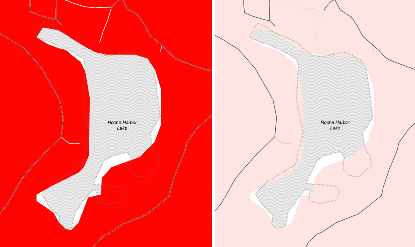
Our original “red” polygons compared to the polygons style with an rgba value.
Notice that the waves of the lake polygon are still blocked by our de-saturated ‘red’.
That’s because the default blend mode of the polygons draw style is opaque. The blend mode defines the way in which color interacts with the underlying layers. Some of the modes, like add and multiply work similarly to Photoshop filters. In our case, opaque is simply opaque, and it obscures all of the underlying features. To make it semi-transparent, we need to set a blend mode of inlay or overlay.
Let’s do this by creating a styles block near the top of our scene file with a single custom style we’ll call _alpha_polygons:
import: https://mapzen.com/carto/refill-style/6/refill-style.zip

styles:
    _alpha_polygons:
        base: polygons
        blend: overlay
This style extends the polygons style we’ve already worked with, but changes the blend mode from the default (opaque) to overlay.
Next, we’ll update our layer with the new style name, _alpha_polygons:
        draw:
            _alpha_polygons:
                order: global.sdk_order_under_roads_0
                color: rgba(255, 0, 0, 0.35)
And reload the map. Much better! The color is still saturated, but now we can (partially) see the waves of the underlying lake polygon.
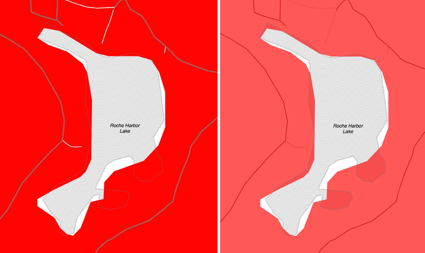
Our original “red” polygons compared to a custom _alpha_polygon style with an rgba value.
Great. Now let’s do something a little more interesting than plain red polygons.
You know, before your patience erodes any further.
JavaScript Functions
Did you know that Tangram’s YAML parser accepts JavaScript functions? I didn’t. Granted, I’m new here, but this was a very exciting realization for me.
We are already filtering out water by using the not filter function. Let’s try replacing that not filter with an equivalent JavaScript function:
        filter:
            all:
                - { $zoom: { min: 10 } }
               - function() { return feature.GLG_SYM != 'water' }
As Tangram parses the YAML file, it will notice the function keyword and treat the text that follows as a JavaScript function. We can even add comments to our function in JavaScript’s own comment syntax:
        filter:
            all:
                - { $zoom: { min: 10 } }
                - |
                    function() {
                        // Filter out water
                        return feature.GLG_SYM != 'water';
                    }
The pipe (|) and newline preceding the function lets the parser know that a multi-line string is coming up. That way, we can write our functions so that they still look like code.
Gneiss!
(I am so sorry.)
Moving on…
Let’s tackle our polygon style, next. I want a different color for each geologic unit on my map, to more or less align with this suggested range of colors from the FGDC.
Lucky for us, Tangram passes our GeoJSON feature properties to all JavaScript functions under the feature keyword.
So instead of passing in a fixed color, we can use JavaScript to return a color based on our GLG_SYM property:
            _alpha_polygons:
                order: global.sdk_order_under_roads_0
                color: |
                    function() {
                        var category = feature.GLG_SYM;
                        var color = category == 'Qa'       ? '#FFF79A' :
                                    category == 'Qb'       ? '#FFF46E' :
                                    category == 'Qd'       ? '#fff377' :
                                    category == 'Qf'       ? '#dddddd' :
                                    category == 'Qp'       ? '#EAC88D' :
                                    category == 'Qgdm'     ? '#FCBB62' :
                                    category == 'Qgdm(es)' ? '#FEE9BB' :
                                    category == 'Qgdm(e)'  ? '#E8A121' :
                                    category == 'Qgom(e)'  ? '#EAB564' :
                                    category == 'Qgom'     ? '#FECE7A' :
                                    category == 'Qgd'      ? '#FEDDA3' :
                                    category == 'Qgt'      ? '#FCBB62' :
                                    category == 'KJmm(c)'  ? '#86C879' :
                                    category == 'KJm(ll)'  ? '#9FD08A' :
                                    category == 'JTRmc(o)' ? '#27BB9D' :
                                    category == 'TRn'      ? '#ED028C' :
                                    category == 'TRPMv'    ? '#F172AC' :
                                    category == 'TRPv'     ? '#F499C2' :
                                    category == 'PDmt'     ? '#40C7F4' :
                                    category == 'pPsh'     ? '#9BA5BE' :
                                    category == 'pDi'      ? '#848FC7' :
                                    category == 'pDit(t)'  ? '#B28ABF' :
                                    '#000';

                        return color;
                    }
Ooh, look at that nice spacing…
Reload the map and check it out.
Look at that, we made a thematic map! This is just a simple categorization, but I bet you can already see how we can use this method for choropleths, proportional symbols, value-by-alpha, and other types of thematic maps.
Well, this is fine, but you know what would make this map even better?
Hillshading!
Whaaaaa?!
Yup. Let’s do this.
Instead of Refill, let’s import Mapzen’s Walkabout style, which comes with a nice built-in hillshade:
import: https://mapzen.com/carto/walkabout-style/3/walkabout-style.zip
Next, we’ll update our custom _alpha_polygons style to use the multiply blend mode:
    _alpha_polygons:
        base: polygons
        blend: multiply
The multiply blend mode multiplies the color of our layer with the underlying layer colors, resulting in a darker color on screen. In this case, I want our geology polygon colors to multiply with the underlying hillshading provided by Walkabout. This will add some very nice texture to our final product.
At this point, our roads are still on top of our polygons. That’s ok but I’d like them to blend in a bit better with our map. So, while we’re making updates, let’s bump up the order of our _geology layer from global.sdk_order_under_roads_0 (the basic underlay) to global.sdk_order_over_everything_but_text_0 (the classic overlay). If you recall from last time, these globals are provided by Mapzen’s basemap styles to make it easier for ordering your own data on a map.
Read more about ordering here. (And don’t worry. Our labels will still be on top!)
Your scene file should now look something like this:
import: https://mapzen.com/carto/walkabout-style/3/walkabout-style.zip

styles:
    _alpha_polygons:
        base: polygons
        blend: multiply

sources:
    _nps_boundary:
        type: GeoJSON
        url: https://gist.githubusercontent.com/rfriberg/684645c22f495b4a46f29fb312b6d268/raw/843ed38a3920ed199082636fe198ba995f5cfc04/san_juan_nhp.geojson

    _nps_geology:
        type: GeoJSON
        url: https://gist.githubusercontent.com/rfriberg/3c09fe3afd642224da7cd70aff1c1e70/raw/1f1df59f4cb4e82d7ea23452c789bc99c299a5cb/san_juan_nhp_geology.geojson

layers:
    _national_park:
        data: { source: _nps_boundary }
        draw:
            lines:
                visible: false
                width: [[8, 0.5px], [18, 5px]]
                color: '#518946'
                order: global.sdk_order_under_roads_1

    _geology:
        data: { source: _nps_geology }
        filter:
            all:
                - { $zoom: { min: 10 } }
                - not: { GLG_SYM: water }
        draw:
            _alpha_polygons:
                order: global.sdk_order_over_everything_but_text_0
                color: |
                    function() {
                        // Note: this is a block of JavaScript so we can use JS comment syntax
                        var category = feature.GLG_SYM;
                        var color = category == 'Qa'       ? '#FFF79A' :
                                    category == 'Qb'       ? '#FFF46E' :
                                    category == 'Qd'       ? '#fff377' :
                                    category == 'Qf'       ? '#dddddd' :
                                    category == 'Qp'       ? '#EAC88D' :
                                    category == 'Qgdm'     ? '#FCBB62' :
                                    category == 'Qgdm(es)' ? '#FEE9BB' :
                                    category == 'Qgdm(e)'  ? '#E8A121' :
                                    category == 'Qgom(e)'  ? '#EAB564' :
                                    category == 'Qgom'     ? '#FECE7A' :
                                    category == 'Qgd'      ? '#FEDDA3' :
                                    category == 'Qgt'      ? '#FCBB62' :
                                    category == 'KJmm(c)'  ? '#86C879' :
                                    category == 'KJm(ll)'  ? '#9FD08A' :
                                    category == 'JTRmc(o)' ? '#27BB9D' :
                                    category == 'TRn'      ? '#ED028C' :
                                    category == 'TRPMv'    ? '#F172AC' :
                                    category == 'TRPv'     ? '#F499C2' :
                                    category == 'PDmt'     ? '#40C7F4' :
                                    category == 'pPsh'     ? '#9BA5BE' :
                                    category == 'pDi'      ? '#848FC7' :
                                    category == 'pDit(t)'  ? '#B28ABF' :
                                    '#000';

                        return color;
                    }
Reload and marvel:
Pretty!
EXTRA CREDIT
I don’t want to take your attention for granite (groan), but let’s make one more change to our map…
Remember our national park boundaries? Let’s add those back into our map, so we can see the outlines over our geology polygons.
In your scene file, update the order so that it’s one above our geology layer and remove the visible: false line that we added at the beginning of this post.
            lines:
                width: [[8, 0.5px], [18, 5px]]
                color: '#518946'
                order: global.sdk_order_over_everything_but_text_1
You should see a simple green line outlining the San Juan National Historic Park. Let’s make those stand out a little more.
Add another custom style to the top of your scene called _dashed_lines:
    _dashed_lines:
        base: lines
        dash: [3, 1]
        dash_background_color: rgb(149, 188, 141)
And update the style name on the national park layer from lines to _dashed_lines:
        draw:
            _dashed_lines:
                width: [[8, 0.5px], [18, 5px]]
                color: '#518946'
                order: global.sdk_order_over_everything_but_text_1
If you couldn’t tell from the code, we changed our plain jane green line into a dashed green line. Oooh! The dash parameter defines the dash pattern we want to use. Here, our [3,1] creates a dash that is 3 times as long as the line’s width, spaced 1 width apart.
The full code for this exercise can be seen on bl.ocks.org. You can also view and modify this scene file in Tangram Play.
Thanks for coming along on another whirlwind tour of mapzen.js and the Tangram scene file. Join us for the next Make Your Own post when we talk about about adding our own labels to the map and overriding features in a Mapzen basemap style.
If you have questions or want to show off something you’ve made with Mapzen, drop us a line. We love to hear from you!
Geologic time scale artwork by Ray Troll, via trollart.com.
Check out additional tutorials from the Make Your Own series:
